

There are nearly endless uses and examples of classification techniques in machine learning. Even the layperson encounters machine learning classification on a regular basis, such as the binary classification involved in spam detection. For those in the field, it is critical to develop a deep, sophisticated understanding of classification techniques in machine learning in order to effectively apply them to business objectives.
In the blog post below, our Artificial Intelligence Research Scientist, Gene Locklear, explains several classification techniques in machine learning and how they might be used successfully.
What Is Classification in Machine Learning?
To get started, what is classification in machine learning? We can describe “classification” as the action or process of assigning a label to an object based on its shared characteristics with a class of objects.
Classification problems can involve any number of “classes,” which are defined as a group containing objects that share common attributes. In binary classification, however, only two classes are allowed.
Binary classification problems are very common. Often, we even take multiple-class classification problems and reduce them to binary classification problems in order to lessen the complexity and computational overhead of the problem.
When we view classification problems in the context of machine learning, we describe them as a supervised learning technique in which our classification algorithm learns from the data it is given. The algorithm then takes what it learns and applies it to data it has not yet seen.
Examining Classification Techniques in Machine Learning
There are many different types of classifiers, from those that involve simple mathematical techniques to those that involve complex mathematics joined with probabilistic selection (ensemble learning).
Next, let’s discuss some simple classification techniques in machine learning and how we can use those techniques to build simple classifiers that can sometimes be sufficient.
Classification in Machine Learning Example: SDi’s REDSUB
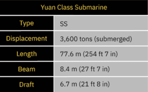
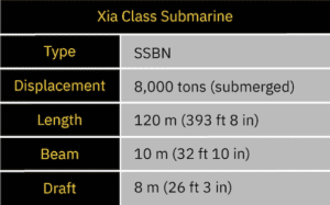
At Sentient Digital, the R&D Department has been tasked with developing a submarine classification system that can identify a Yuan-class diesel-electric submarine from a Xia-class nuclear-powered ballistic missile submarine. To provide a solution for this task, SDi has created REDSUB.
REDSUB is equipped with a variety of static underwater sensors that can perceive the length, beam, and draft of a passing submarine. These sensors can also detect disturbances in the surrounding water column caused by the submarine’s propulsion system and hull composition. REDSUB records this information about each submarine it detects.
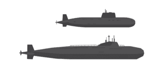
The sensor array that composes REDSUB is affected by the speed and distance of the submarine as well as a variety of environmental factors. Thus, while we can see from a simple, clear observation that these submarines are quite different, the sensor array isn’t always able to get a complete and clear observation. This limitation prevents a definitive classification of a submarine based on a single observation.
Over time, REDSUB has amassed a data set of sensor observations for each type of submarine under a variety of environmental conditions. For each one of these observations, human intelligence and satellite imagery has labeled what the actual type of submarine was for that observation. This correctly labeled data, known as our “training data set,” will be what is used to train our classification systems.
REDSUB’s Training Data Set
We receive the data collected by REDSUB for verified submarine detections in the format below. Each row is a single verified detection, and the values are what each sensor reported about the detection. Each row is a specific sensor recording for the specified detection. In aggregate, they represent how REDSUB sees either a Yuan- or Xia-class submarine.
| Class | Estimated Length | Estimated Beam | Estimated Draft | Pressure Change | Vortex Duration | Magnetic Disruption | Light Refraction |
|---|---|---|---|---|---|---|---|
| Yuan | 62.08 | 7.96 | 5.03 | 534.56 | 965.18 | 17.21 | 0.94 |
| Yuan | 73.72 | 8.40 | 6.37 | 835.25 | 463.29 | 15.49 | 1.06 |
| Yuan | 77.60 | 6.30 | 6.70 | 890.93 | 463.29 | 17.21 | 0.56 |
| Yuan | 77.60 | 6.72 | 5.03 | 534.56 | 463.29 | 13.77 | 0.56 |
| Yuan | 69.84 | 6.72 | 5.36 | 1113.67 | 965.18 | 8.26 | 1.06 |
| Class | Estimated Length | Estimated Beam | Estimated Draft | Pressure Change | Vortex Duration | Magnetic Disruption | Light Refraction |
|---|---|---|---|---|---|---|---|
| Xia | 96.00 | 4.80 | 6.40 | 3157.92 | 1697.28 | 57.60 | 14.40 |
| Xia | 96.00 | 8.00 | 6.00 | 3508.80 | 1909.44 | 51.84 | 14.40 |
| Xia | 57.60 | 4.80 | 7.20 | 3157.92 | 1909.44 | 43.20 | 14.40 |
| Xia | 114.00 | 4.80 | 7.60 | 3333.36 | 1697.28 | 54.72 | 17.10 |
| Xia | 90.00 | 9.00 | 7.60 | 2631.60 | 1018.37 | 43.20 | 16.20 |
Our Use of the Feature Vector for Classification in Machine Learning
With the information in this format for each observation/detection by REDSUB, we created a feature vector to use with our classifier. The feature vector is an array in which the values represent the readings of each of the sensors available to REDSUB.
| Class | Estimated Length | Estimated Beam | Estimated Draft | Pressure Change | Vortex Duration | Magnetic Disruption | Light Refraction |
|---|---|---|---|---|---|---|---|
| The actual class of the submarine | Recording by Sensor_A | Recording by Sensor_B | Recording by Sensor_C | Recording by Sensor_D | Recording by Sensor_E | Recording by Sensor_F | Recording by Sensor_G |
| Class | Estimated Length | Estimated Beam | Estimated Draft | Pressure Change | Vortex Duration | Magnetic Disruption | Light Refraction |
|---|---|---|---|---|---|---|---|
| Yuan | 62.00 | 87.98 | 5.03 | 534.56 | 965.18 | 17.21 | 0.94 |
| Xia | 96.00 | 4.80 | 6.40 | 3157.92 | 1697.28 | 57.60 | 14.40 |
For each submarine class, the training data set contains multiple feature vectors. Taken together, these feature vectors represent the total variation in how the REDSUB sensors perceived that class of submarine under different environmental conditions.
The difference between the sensor-perceived data and what we know about the submarine classes (our ground truth) forces us to consolidate the observations so that we can understand the variance in REDSUB’s sensors.
Even though we know the actual dimensions of the submarines, this “sensor variance” (or sensor accuracy) requires that we build a sensor-oriented model based on the data. This allows us to see how the sensor views each submarine, which may be substantially different than the ground truth, an important distinction to understand in our classification in machine learning example.
Normalization of Feature Vectors
Because the range of values for each feature is so disparate, we need to standardize the values of each feature in each feature vector so that all values conform to some standard scale. There are many approaches to this, but in our classification in machine learning example, we will use z-score normalization.
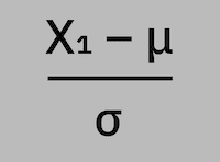
Z-score normalization is the process of normalizing every value in a dataset such that the mean of all the values is 0 and the standard deviation is 1.
Z-score normalization is performed by calculating the mean and standard deviation of the feature vector values, and then subtracting the mean from each value and dividing the difference by the standard deviation: (x1 – μ) / σ
| Original | |||||||
|---|---|---|---|---|---|---|---|
| Class | Estimated Length | Estimated Beam | Estimated Draft | Pressure Change | Vortex Duration | Magnetic Disruption | Light Refraction |
| Yuan | 62.00 | 87.98 | 5.03 | 534.56 | 965.18 | 17.21 | 0.94 |
| Normalized | |||||||
|---|---|---|---|---|---|---|---|
| Class | Estimated Length | Estimated Beam | Estimated Draft | Pressure Change | Vortex Duration | Magnetic Disruption | Light Refraction |
| Yuan | -0.472 | -0.627 | -0.635 | 0.876 | 2.106 | -0.6 | -0.647 |
| Class | Estimated Length | Estimated Beam | Estimated Draft | Pressure Change | Vortex Duration | Magnetic Disruption | Light Refraction |
|---|---|---|---|---|---|---|---|
| Yuan | -0.472 | -0.627 | -0.635 | 0.876 | 2.106 | -0.6 | -0.647 |
| Yuan | -0.42 | -0.637 | -0.644 | 2.105 | 0.871 | -0.614 | -0.661 |
| Yuan | -0.413 | -0.637 | -0.635 | 2.143 | 0.799 | -0.602 | -0.655 |
| Yuan | -0.366 | -0.69 | -0.698 | 1.729 | 1.402 | -0.658 | -0.719 |
| Yuan | -0.518 | -0.654 | -0.657 | 1.734 | 1.413 | -0.651 | -0.667 |
| Class | Estimated Length | Estimated Beam | Estimated Draft | Pressure Change | Vortex Duration | Magnetic Disruption | Light Refraction |
|---|---|---|---|---|---|---|---|
| Xia | -0.542 | -0.622 | -0.62 | 2.122 | 0.851 | -0.576 | -0.613 |
| Xia | -0.549 | -0.617 | -0.619 | 2.114 | 0.866 | -0.583 | -0.612 |
| Xia | -0.579 | -0.624 | -0.622 | 2.045 | 0.988 | -0.592 | -0.616 |
| Xia | -0.527 | -0.618 | -0.615 | 2.153 | 0.791 | -0.576 | -0.608 |
| Xia | -0.496 | -0.584 | -0.586 | 2.274 | 0.516 | -0.547 | -0.577 |
Creating Feature Templates
After we apply normalizations to the feature vectors, we must try to decide on how the feature vector represents the ground truth regarding the way in which REDSUB sensors perceive each submarine they detect.
Because we have a variety of observations, all of which give us a different description of each class of submarine, we need to create an aggregated representation for each class. We refer to this representation as a “template” or “mean” feature vector.
The template is constructed by averaging all the values of each normalized feature for each observation and arriving at a mean for each feature vector value.
| Class | Estimated Length | Estimated Beam | Estimated Draft | Pressure Change | Vortex Duration | Magnetic Disruption | Light Refraction |
|---|---|---|---|---|---|---|---|
| Yuan | -0.472 | -0.627 | -0.635 | 0.876 | 2.106 | -0.6 | -0.647 |
| Yuan | -0.42 | -0.637 | -0.644 | 2.105 | 0.871 | -0.614 | -0.661 |
| Yuan | -0.413 | -0.637 | -0.635 | 2.143 | 0.799 | -0.602 | -0.655 |
| Yuan | -0.366 | -0.69 | -0.698 | 1.729 | 1.402 | -0.658 | -0.719 |
| Yuan | -0.518 | -0.654 | -0.657 | 1.734 | 1.413 | -0.651 | -0.667 |
| Yuan Template | |||||||
|---|---|---|---|---|---|---|---|
| Class | Estimated Length | Estimated Beam | Estimated Draft | Pressure Change | Vortex Duration | Magnetic Disruption | Light Refraction |
| Yuan | -0.438 | -0.649 | -0.654 | 1.717 | 1.318 | -0.625 | -0.67 |
| Class | Estimated Length | Estimated Beam | Estimated Draft | Pressure Change | Vortex Duration | Magnetic Disruption | Light Refraction |
|---|---|---|---|---|---|---|---|
| Xia | -0.542 | -0.622 | -0.62 | 2.122 | 0.851 | -0.576 | -0.613 |
| Xia | -0.549 | -0.617 | -0.619 | 2.114 | 0.866 | -0.583 | -0.612 |
| Xia | -0.579 | -0.624 | -0.622 | 2.045 | 0.988 | -0.592 | -0.616 |
| Xia | -0.527 | -0.618 | -0.615 | 2.153 | 0.791 | -0.576 | -0.608 |
| Xia | -0.496 | -0.584 | -0.586 | 2.274 | 0.516 | -0.547 | -0.577 |
| Xia Template | |||||||
|---|---|---|---|---|---|---|---|
| Class | Estimated Length | Estimated Beam | Estimated Draft | Pressure Change | Vortex Duration | Magnetic Disruption | Light Refraction |
| Xia | -0.539 | -0.613 | -0.613 | 2.142 | 0.802 | -0.575 | -0.605 |
Simple Classifier Types and Classification Techniques in Machine Learning
Now that we have data in a form that is most useful to us, we can think about some simple classifiers and classification techniques in machine learning that we might use.
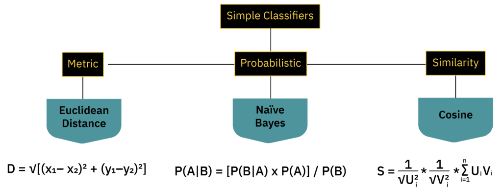
Metric Classification in Machine Learning
A metric is a function that maps a distance between a set of points. We can think of the process of applying the metric as creating a “metric space.” There are many types of metrics, but any metric we create must obey three rules:
- Rule 1: The distance between a point and itself must be 0.
- Rule 2: The distance between Point A and Point B must be the same as the distance between Point B and Point A.
- Rule 3: The distance between Point A and Point B must be less than or equal to the sum of the distance between Points A and Z and the distance between B and Z.
Compared to other classification techniques in machine learning, metric classifiers use some form of distance measure to determine how far apart two classes are. Combined with an acceptance threshold, these classifiers determine whether two feature vectors are close enough to be considered the same class.
Probabilistic Classification in Machine Learning
Probability concerns a numerical explanation of how likely an event is to occur or for some condition to be true. Any event or condition has a probability between 0 and 1 of occurring/being true, where 0 means it never occurs/is never true and 1 means it will occur/is true.
Probabilistic classifiers given an input (some event or condition) and a probability distribution (a mapping of how likely it is for the event/condition to occur/be true). This will return a numerical representation of the likelihood (probability) that the event/condition will occur/be true.
Similarity Classification in Machine Learning
Similarity is a degree of likenesses between two things. A similarity measure is a real-valued mapping between two objects which quantifies how similar these objects are to each other. Similarity has no definitive meaning, but is defined based on a measure of equality among the features that describe the object.
Unlike metric or probabilistic classification techniques in machine learning, similarity classifiers use some form of similarity measure to determine how similar two classes are. Combined with an acceptance threshold, these classifiers determine whether two feature vectors are similar enough to be considered the same class.
Returning to Our Classification in Machine Learning Example
The Euclidean Distance Classifier
Euclidean distance is a metric classifier because it uses the Euclidean distance as the measure of difference between two feature vectors. In our REDSUB example, we have a feature vector of seven dimensions, so our distance formula is: D = √ (F₁₁ – F₂₁)² + (F₁₂ – F₂₂)² + . . . + (F₁₇ – F₂₇)²

The classifier works by calculating the distance between every feature vector in the training data set and the template. This allows us to establish a threshold for distance that is acceptable to classify each type of submarine.
The threshold represents the maximum distance that a feature vector can be from the template and still be classified as a specific class of submarine.
| Yuan Data Set | |||||||
|---|---|---|---|---|---|---|---|
| Class | Estimated Length | Estimated Beam | Estimated Draft | Pressure Change | Vortex Duration | Magnetic Disruption | Light Refraction |
| Yuan | -0.472 | -0.627 | -0.635 | 0.876 | 2.106 | -0.6 | -0.647 |
| Yuan | -0.42 | -0.637 | -0.644 | 2.105 | 0.871 | -0.614 | -0.661 |
| Yuan | -0.413 | -0.637 | -0.635 | 2.143 | 0.799 | -0.602 | -0.655 |
| Yuan | -0.366 | -0.69 | -0.698 | 1.729 | 1.402 | -0.658 | -0.719 |
| Yuan | -0.518 | -0.654 | -0.657 | 1.734 | 1.413 | -0.651 | -0.667 |
| Yuan Template | |||||||
|---|---|---|---|---|---|---|---|
| Class | Estimated Length | Estimated Beam | Estimated Draft | Pressure Change | Vortex Duration | Magnetic Disruption | Light Refraction |
| Yuan | -0.438 | -0.649 | -0.654 | 1.717 | 1.318 | -0.625 | -0.67 |
| Euclidean Distances | |||||
|---|---|---|---|---|---|
| Class | 1 | 2 | 3 | 4 | 5 |
| Yuan | 1.153 | 0.592 | 0.673 | 0.14 | 0.128 |
| Threshold is 1.153 |
| Xia Data Set | |||||||
|---|---|---|---|---|---|---|---|
| Class | Estimated Length | Estimated Beam | Estimated Draft | Pressure Change | Vortex Duration | Magnetic Disruption | Light Refraction |
| Xia | -0.542 | -0.622 | -0.62 | 2.122 | 0.851 | -0.576 | -0.613 |
| Xia | -0.549 | -0.617 | -0.619 | 2.114 | 0.866 | -0.583 | -0.612 |
| Xia | -0.579 | -0.624 | -0.622 | 2.045 | 0.988 | -0.592 | -0.616 |
| Xia | -0.527 | -0.618 | -0.615 | 2.153 | 0.791 | -0.576 | -0.608 |
| Xia | -0.496 | -0.584 | -0.586 | 2.274 | 0.516 | -0.547 | -0.577 |
| Xia Template | |||||||
|---|---|---|---|---|---|---|---|
| Class | Estimated Length | Estimated Beam | Estimated Draft | Pressure Change | Vortex Duration | Magnetic Disruption | Light Refraction |
| Xia | -0.539 | -0.613 | -0.613 | 2.142 | 0.802 | -0.575 | -0.605 |
| Euclidean Distances | |||||
|---|---|---|---|---|---|
| Class | 1 | 2 | 3 | 4 | 5 |
| Xia | 0.054 | 0.071 | 0.215 | 0.021 | 0.324 |
| Threshold is 0.324 |
Once we have established the threshold for each class, we can use those thresholds to classify observations that our classifier has not yet seen.
| F1 | F2 | F3 | F4 | F5 | F6 | F7 | |
|---|---|---|---|---|---|---|---|
| Class | Estimated Length | Estimated Beam | Estimated Draft | Pressure Change | Vortex Duration | Magnetic Disruption | Light Refraction |
| UNKNOWN | 77 | 11.00 | 7 | 3200.00 | 2900.00 | 48.00 | 14.00 |
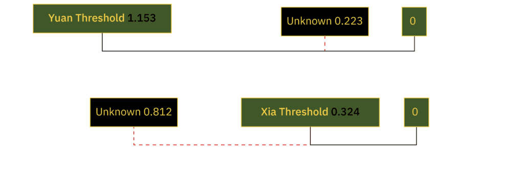
Thus, we can see that our Euclidean distance classifier shows the Yuan class to be closer to the UNKNOWN class than the Xia.
The Naive Bayes Classifier
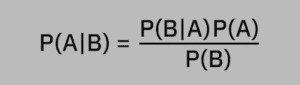
Naive Bayes is a conditional probability classifier that, when given the feature vector to be classified, calculates a probability that the feature vector belongs to one of a specified number of classes. The Naive Bayes classifier relies on the use of Bayes’ theorem that states: P(A|B) = [P(B|A) x P(A)] / P(B)
Where:
P(A|B) is the conditional probability that specifies the probability that A is true given that B is also true. We refer to this as the “posterior probability.”
P(B|A) is the conditional probability that specifies the probability that B is true given that A is also true. We refer to this as the “likelihood.”
P(A) is just the probability that A is true.
P(B) is just the probability that B is true.
The Naive Bayes classifier relies on the assumption that there is no correlation between the individual values of the feature vector. We can state this simply as each feature is independent of every other feature in the feature vector.
REDSUB and Naive Bayes Classification Techniques in Machine Learning
In our machine learning classification example, we need REDSUB to be able to distinguish its detections as either a Yuan-class or Xia-class submarine. Thus, we have two classes: either Yuan or Xia.
Unlike our previous example, we are not normalizing our data set to train our Naive Bayes classifier because each of the feature values are treated individually. Our first step in constructing the classifier is to conduct some statistical analysis of our data set so that we can get the values that we need for our classifier.
| Class | Estimated Length | Estimated Beam | Estimated Draft | Pressure Change | Vortex Duration | Magnetic Disruption | Light Refraction |
|---|---|---|---|---|---|---|---|
| Yuan | 62.08 | 7.96 | 5.03 | 534.56 | 965.18 | 17.21 | 0.94 |
| Yuan | 73.72 | 8.40 | 6.37 | 835.25 | 463.29 | 15.49 | 1.06 |
| Yuan | 77.60 | 6.30 | 6.70 | 890.93 | 463.29 | 17.21 | 0.56 |
| Yuan | 77.60 | 6.72 | 5.03 | 534.56 | 463.29 | 13.77 | 0.56 |
| Yuan | 69.84 | 6.72 | 5.36 | 1113.67 | 965.18 | 8.26 | 1.06 |
| Class | Estimated Length | Estimated Beam | Estimated Draft | Pressure Change | Vortex Duration | Magnetic Disruption | Light Refraction |
|---|---|---|---|---|---|---|---|
| Xia | 96.00 | 4.80 | 6.40 | 3157.92 | 1697.28 | 57.60 | 14.40 |
| Xia | 96.00 | 8.00 | 6.00 | 3508.80 | 1909.44 | 51.84 | 14.40 |
| Xia | 57.60 | 4.80 | 7.20 | 3157.92 | 1909.44 | 43.20 | 14.40 |
| Xia | 114.00 | 4.80 | 7.60 | 3333.36 | 1697.28 | 54.72 | 17.10 |
| Xia | 90.00 | 9.00 | 7.60 | 2631.60 | 1018.37 | 43.20 | 16.20 |
In the chart below, we calculate the mean and variance for each individual feature in the feature vector.
| Class | Mean | Variance | Mean | Variance | Mean | Variance | Mean | Variance | Mean | Variance | Mean | Variance | Mean | Variance |
|---|---|---|---|---|---|---|---|---|---|---|---|---|---|---|
| Length | Beam | Draft | Pressure | Vortex | Magnetic | Light | ||||||||
| Yuan | 72.68 | 42.15 | 7.22 | 0.82 | 5.69 | 0.61 | 781.79 | 61789.79 | 664.04 | 75568.09 | 14.38 | 13.76 | 0.83 | 0.06 |
| Xia | 90.72 | 423.79 | 6.28 | 4.23 | 6.96 | 0.52 | 3157.92 | 107727.17 | 1646.36 | 134494.82 | 50.11 | 43.96 | 15.3 | 1.62 |
Next, because we are assuming that our observations come from a set of observations which have a normal distribution and that the value of each feature is continuous, we will calculate the probability using the Gaussian probability density function.
A probability density function (PDF) is used to define the random variable’s probability of being within a distinct range of values, as opposed to taking on any one value: p (Fᵢ) = 1 / (√2πσ²) * e^ [– (x–μ)² / 2σ²]

Classifying a New REDSUB Observation with Our Naive Bayes Classifier
Let’s suppose we get a new observation by REDSUB, and we want to use our Naive Bayes classifier to determine its class.
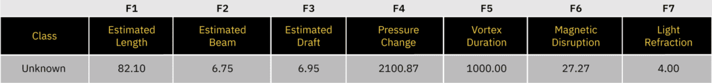
| F1 | F2 | F3 | F4 | F5 | F6 | F7 | |
|---|---|---|---|---|---|---|---|
| Class | Estimated Length | Estimated Beam | Estimated Draft | Pressure Change | Vortex Duration | Magnetic Disruption | Light Refraction |
| UNKNOWN | 82.10 | 6.75 | 6.95 | 2100.87 | 1000.00 | 27.27 | 4.00 |
Our Naive Bayes classifier utilizes Bayes’ theorem combined with a decision-making process. Most commonly, we choose this process to be the maximum a posteriori (MAP) selection process. This process works by calculating the posterior for each possible class.
Posterior is just the conditional probability given that we had some previous information. It can be stated simply as the probability after all known evidence is considered:
Posteriorᵧᵤₐₙ Cₗₐₛₛ = [P(Yuan)P(F1|Yuan)P(F2|Yuan)P(F3|Yuan)P(F4|Yuan)P(F5|Yuan)P(F6|Yuan)P(F7|Yuan)] / Evidence
Posteriorₓᵢₐ Cₗₐₛₛ = [P(Xia)P(F1|Xia)P(F2|Xia)P(F3|Xia)P(F4|Xia)P(F5|Xia)P(F6|Xia)P(F7|Xia)] / Evidence
Evidence = P(Yuan)P(F1|Yuan)P(F2|Yuan)P(F3|Yuan)P(F4|Yuan)P(F5|Yuan)P(F6|Yuan)P(F7|Yuan) + P(Xia)P(F1|Xia)P(F2|Xia)P(F3|Xia)P(F4|Xia)P(F5|Xia)P(F6|Xia)P(F7|Xia)
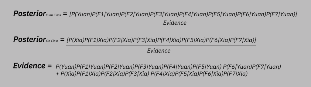
Because the evidence (in this data set) is a constant and is the same for both Yuan and Xia class, we can simply exclude it from our calculations.
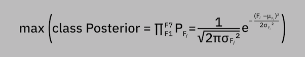
For us to classify the new observation, we calculate the posterior value for each feature in the feature vector and take the product of those values. The class with the highest posterior product (maximum a posteriori) is the class we select: max (class Posterior = ∏F⁷F1 PFᵢ = 1 / (√2πσFᵢ²) * e^ [– (Fᵢ–μFᵢ)² / 2σFᵢ²]
| F1 | F2 | F3 | F4 | F5 | F6 | F7 | |
|---|---|---|---|---|---|---|---|
| Class | Estimated Length | Estimated Beam | Estimated Draft | Pressure Change | Vortex Duration | Magnetic Disruption | Light Refraction |
| UNKNOWN | 82.10 | 6.75 | 6.95 | 2100.87 | 1000.00 | 27.27 | 4.00 |
| Yuan Class | Xia Class | ||||||||||
|---|---|---|---|---|---|---|---|---|---|---|---|
| Feature | Class | New Observation | Gaussian PDF Value | Feature | Class | New Observation | Gaussian PDF Value | ||||
| Mean | Variance | Mean | Variance | ||||||||
| F1 | 72.16 | 42.15 | 82.10 | 1.907E-2 | F1P | F1 | 90.720 | 423.792 | 82.10 | 1.775E-2 | F1P |
| F2 | 7.22 | 0.82 | 6.75 | 38.26E-2 | F2P | F2 | 6.280 | 4.232 | 6.75 | 18.89E-2 | F2P |
| F3 | 5.69 | 0.61 | 6.95 | 14.23E-2 | F3P | F3 | 6.960 | 0.528 | 6.95 | 54.9E-2 | F3P |
| F4 | 781.79 | 61789.79 | 2100.87 | 12.32E-10 | F4P | F4 | 3157.920 | 107727.178 | 2100.87 | 6.80E-6 | F4P |
| F5 | 664.04 | 75568.07 | 1000.00 | 6.877E-4 | F5P | F5 | 1646.362 | 134494.825 | 1000.00 | 2.302E-4 | F5P |
| F6 | 14.38 | 13.76 | 27.27 | 2.596E-4 | F6P | F6 | 50.112 | 43.960 | 27.27 | 1.593E-4 | F6P |
| F7 | 0.83 | 0.06 | 4.00 | 15.66E-34 | F7P | F7 | 15.300 | 1.620 | 4.00 | 2.401E-18 | F7P |
| Yuan Posterior | F1P x F2P x F3P x F4P x F5P x F6P x F7P | Xia Posterior | F1P x F2P x F3P x F4P x F5P x F6P x F7P | ||||||||
| 3.577E-52 | 11.02E-34 | ||||||||||
Thus, we can see that our Naive Bayes classifier chooses Xia class.
Using Cosine Similarity
Cosine similarity is a similarity between two feature vectors of an inner product space. This inner product space is defined to be equal to the cosine of the angle between the two feature vectors. This can be considered the same as the inner product of the feature vectors where their lengths are both normalized to 1.
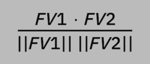
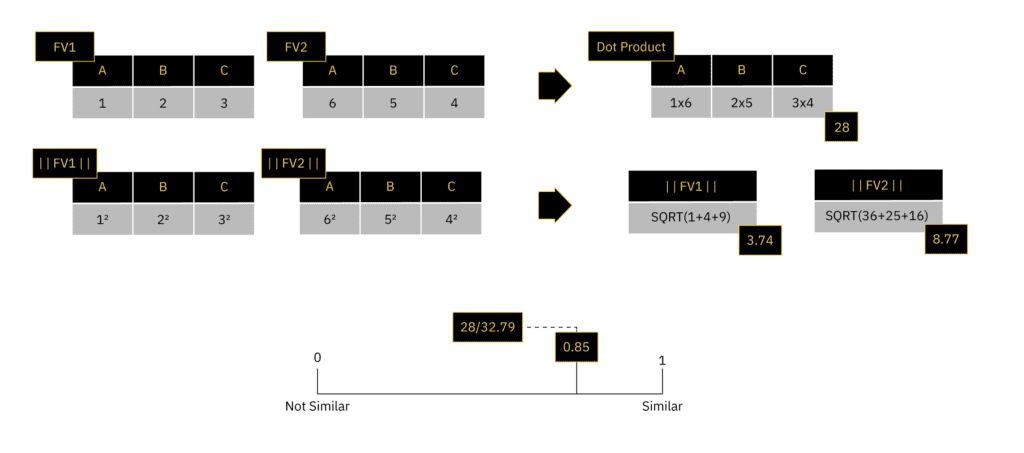
The cosine of two feature vectors can be derived by using the Euclidean dot product formula. This can be simply stated as the sum of the products of the individual values of the feature vectors (dot product) divided by the product of the magnitudes of each feature vector. We can write this in vector form as: (FV1 * FV2) / (||FV1|| ||FV2||)
The cosine similarity is bounded in the interval [-1,1] for any angle. However, we will consider only positive space where it is bounded [0,1]. Two feature vectors with the same orientation have a cosine similarity of 1; two feature vectors oriented at a right angle relative to each other have a similarity of 0.
A Simple Example of Cosine Similarity with REDSUB
In the example above, the classifier works by calculating the cosine similarity between every feature vector in the training data set and the template. This allows us to establish a threshold for a similarity that is acceptable to classify each type of submarine. The threshold represents the minimum similarity a feature vector must have to the template and still be classified as a specific class of submarine.
| Yuan Data Set | |||||||
|---|---|---|---|---|---|---|---|
| Class | Estimated Length | Estimated Beam | Estimated Draft | Pressure Change | Vortex Duration | Magnetic Disruption | Light Refraction |
| Yuan | -0.472 | -0.627 | -0.635 | 0.876 | 2.106 | -0.6 | -0.647 |
| Yuan | -0.42 | -0.637 | -0.644 | 2.105 | 0.871 | -0.614 | -0.661 |
| Yuan | -0.413 | -0.637 | -0.635 | 2.143 | 0.799 | -0.602 | -0.655 |
| Yuan | -0.366 | -0.69 | -0.698 | 1.729 | 1.402 | -0.658 | -0.719 |
| Yuan | -0.518 | -0.654 | -0.657 | 1.734 | 1.413 | -0.651 | -0.667 |
| Yuan Template | |||||||
|---|---|---|---|---|---|---|---|
| Class | Estimated Length | Estimated Beam | Estimated Draft | Pressure Change | Vortex Duration | Magnetic Disruption | Light Refraction |
| Yuan | -0.438 | -0.649 | -0.654 | 1.717 | 1.318 | -0.625 | -0.67 |
| Similarity | |||||
|---|---|---|---|---|---|
| Class | 1 | 2 | 3 | 4 | 5 |
| Yuan | 0.902 | 0.975 | 0.967 | 0.999 | 0.999 |
| Threshold is 0.902 |
| Class | Estimated Length | Estimated Beam | Estimated Draft | Pressure Change | Vortex Duration | Magnetic Disruption | Light Refraction |
|---|---|---|---|---|---|---|---|
| Xia | -0.542 | -0.622 | -0.62 | 2.122 | 0.851 | -0.576 | -0.613 |
| Xia | -0.549 | -0.617 | -0.619 | 2.114 | 0.866 | -0.583 | -0.612 |
| Xia | -0.579 | -0.624 | -0.622 | 2.045 | 0.988 | -0.592 | -0.616 |
| Xia | -0.527 | -0.618 | -0.615 | 2.153 | 0.791 | -0.576 | -0.608 |
| Xia | -0.496 | -0.584 | -0.586 | 2.274 | 0.516 | -0.547 | -0.577 |
| Xia Template | |||||||
|---|---|---|---|---|---|---|---|
| Class | Estimated Length | Estimated Beam | Estimated Draft | Pressure Change | Vortex Duration | Magnetic Disruption | Light Refraction |
| Xia | -0.539 | -0.613 | -0.613 | 2.142 | 0.802 | -0.575 | -0.605 |
| Similarity | |||||
|---|---|---|---|---|---|
| Class | 1 | 2 | 3 | 4 | 5 |
| Xia | 0.99978 | 0.99963 | 0.99670 | 0.99997 | 0.99250 |
| Threshold is 0.992 |
Cosine similarity conducts classification in a binary fashion: observation is either similar enough or not.
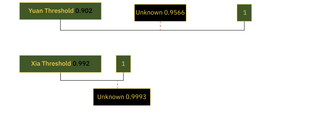
When calculating the cosine similarity between each of the submarine class templates and the UNKNOWN observation, we see that the observation is well within the threshold of either class. Our first thought might be that it is much closer in similarity to the Xia class than the Yuan class.
However, while we could use such a criterion for deciding, we must be careful in doing so. Most likely, what this tells us is that there is insufficient discrimination between the two classes when using cosine similarity.
We either need better data that contains more discriminatory variables (features) or the cosine similarity technique is just insufficient mathematically (too simple) to discern the difference. This is a common classification problem in machine learning. It is why we must often use much more advanced mathematics than the ones used in these simple classifiers.
Final Thoughts on Our REDSUB Classification in Machine Learning Example
Classification is a difficult but common machine learning problem. There is no one accepted approach to associate classification techniques in machine learning with problem types. Instead, we just use repeated model evaluation and refinement to discover which techniques lead to the best results for a given classification task.
Classification models will never provide perfect results. But a model with a high accuracy can best be achieved many times by starting with a simple concept and first discovering whether the problem lies in either the data or the mathematical approach. This is a good first step before moving on to more mathematically intense and computationally expensive approaches.
Join Our Team to Work with Classification Techniques in Machine Learning
Sentient Digital is always on the lookout for promising new talent. If you are interested in working with classification techniques in machine learning and other innovative strategies, technologies, and solutions, browse our current job postings or contact us today to talk about a career at SDi.