

With any significant investment, it is critical that an organization can measure its results accurately and productively. This is especially true for machine learning systems. Whether it’s a pre-made software, no code or low code platform, or customized solution, machine learning can be improved through available data and experiences. Learning how to interpret machine learning results is not only important for justifying its investment to stakeholders, but also potentially improving its performance.
In the blog post below, our Artificial Intelligence Research Scientist, Gene Locklear, explains how to analyze test results meaningfully for a machine learning system.
How to Interpret Machine Learning Results Using Measures of Effectiveness
Measures of Effectiveness (MOE) are metrics constructed to quantify the results of some system or process. They are generally expressed (in scientific terms) as probabilities.
We can think of MOE as a series of binary outputs that are associated with some probability of occurring:
- Does the system do what it was intended to do?
- Does the system do what it should do?
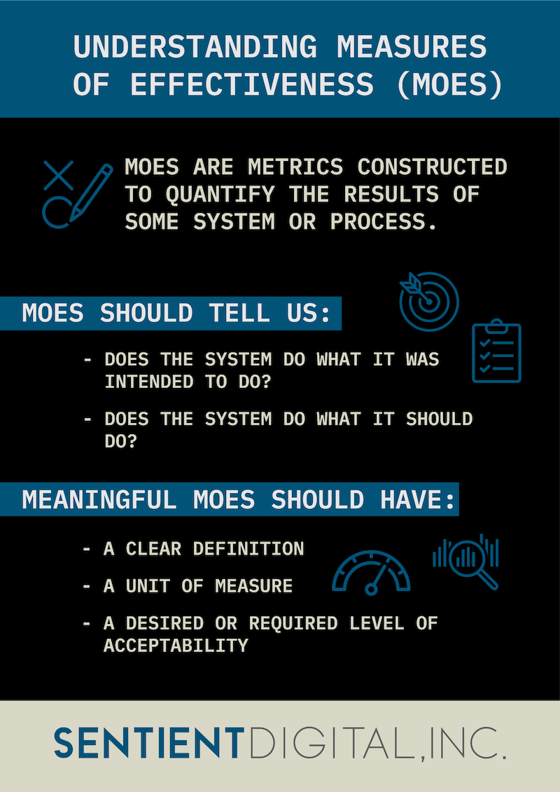 Choosing the right MOEs is a critical step in learning how to interpret machine learning results. An MOE should have a clear definition (for example, “Detects hostile targets”), a unit of measure (“Percentage of hostile targets detected”), a desired or required level of acceptability (“Detection rate is 90%”), and how the level of acceptability affects the overall MOE.
Often, we may consider the use of simple calculations as an effective MOE. For instance, if the system was right 8 out 10 times, it has an 80% effectiveness. However, this is a very misleading way to think about measuring how well a system is performing.
Consider This Example of a Misleading MOE
The R&D Department at Sentient Digital has developed a software program, SUB_BUSTER, that allows autonomous underwater drones to detect and target hostile submarines. After a series of simulation trials, it was shown that SUB_BUSTER performed correctly in 53% of all encounters.
We could state this by saying that SUB_BUSTER is correct 53% of the time when it indicates that a submarine is hostile and that it is wrong 47% of the time. The 53% of the time that SUB_BUSTER was wrong, it either indicated that a submarine was hostile and it wasn’t, or it indicated that it wasn’t hostile and it was.
This statement—that SUB_BUSTER has a 53% effectiveness—really means that when testing SUB_BUSTER, it correctly identified roughly 5 out of 10 submarines that were hostile as being hostile. This is a useful metric of the effectiveness of SUB_BUSTER, but far from a totally adequate one.
Imagine there is a detector that classified every submarine by default as hostile. It would be 100% effective when identifying hostile submarines. The problem, of course, is that it would also classify friendly submarines as hostile. Therefore, this is not a reliable indicator of whether any individual submarine was hostile or not.
Relying on a misleading MOE such as this is a common issue in understanding how to interpret machine learning results. Because there is ambiguity in the statement about SUB_BUSTER’s actual effectiveness, we want a more thorough analysis that will provide a better explanation of how effective SUB_BUSTER is.
How to Interpret Machine Learning Results Effectively for SUB_BUSTER
Let’s examine SUB_BUSTER’s test results and dissect each part.
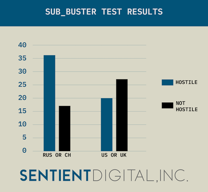
SUB_BUSTER Test Results
In the simulation:
- SUB_BUSTER encountered 100 submarines.
- 53 of the submarines were from Russia or China (Yasen Class or Changzheng Class).
- 47 of the submarines were from the U.S. or U.K. (OHIO Class, SEAWOLF Class, TRAFALGAR Class, or ASTUTE Class).
Thus, the first thing that we can say about the test is that the prevalence of hostile submarines is 53%. Prevalence tells us the probability of SUB_BUSTER encountering a submarine that is hostile and is very important when adjusting the test results to the actual test conditions.
SUB_BUSTER Test Raw Data
Next, we examine the actual raw data from the test:
- 36 times SUB_BUSTER correctly identified a submarine as hostile when it was a hostile submarine. These are known as true positives.
- 27 times SUB_BUSTER correctly identified a submarine as not hostile when it was not a hostile submarine. These are known as true negatives.
- 20 times SUB_BUSTER incorrectly identified a submarine as hostile when it was not a hostile submarine. These are known as false positives.
- 17 times SUB_BUSTER incorrectly identified a submarine as not hostile when it was a hostile submarine. These are known as false negatives.
We can represent this data in chart form (below), and we refer to this chart as a Confusion Matrix. We can think of a Confusion Matrix as a tabular visualization of how well SUB_BUSTER performed for each type of situation it encountered.
 In our case, SUB_BUSTER has only two situations (known as Classes): either a submarine is hostile or it is not. This defines the decisions that SUB_BUSTER makes as “specific” and identifies SUB_BUSTER as a Binary Classification System (i.e., only two classes allowed).
MOE Indicators for SUB_BUSTER
The values true positive, true negative, false positive, and false negatives give rise to another group of quantifications that specify how effective SUB_BUSTER was:
True Positive Rate (TPR) — The ratio of times when SUB_BUSTER indicated that a submarine was hostile and the submarine was hostile. This is known as SUB_BUSTER’s True Positive Rate or its Sensitivity. TPR is calculated by dividing the number of hostile submarines by the number of times SUB_BUSTER indicated it was hostile.
True Negative Rate (TNR) — The ratio of times when SUB_BUSTER indicated that a submarine was not hostile and the submarine was not hostile. This is known as SUB_BUSTER’s True Negative Rate or its Specificity. TNR is calculated by dividing the number of friendly submarines by the number of times SUB_BUSTER indicated it was not hostile.
False Positive Rate (FPR) — The ratio of times when SUB_BUSTER indicated that a submarine was hostile and the submarine was not hostile. This is known as SUB_BUSTER’s False Positive Rate. FPR is calculated by dividing the number of friendly submarines by the number of times SUB_BUSTER indicated that it was hostile.
False Negative Rate (FNR) — The ratio of times when SUB_BUSTER indicated that a submarine was not hostile and the submarine was hostile. This is known as SUB_BUSTER’s False Negative Rate. FNR is calculated by dividing the number of hostile submarines by the number of times SUB_BUSTER indicated that it was not hostile.
Positive Predictive Value (PPV) — This is a value that represents the probability that SUB_BUSTER will correctly identify a hostile submarine as hostile. PPV is calculated by dividing the number of times SUB_BUSTER was correct about hostile submarines divided by the sum of the number of times it was right about hostile submarines and number of times it misidentified a friendly submarine as being hostile.
Negative Predictive Value (NPV) — This is a value that represents the probability that SUB_BUSTER will correctly identify a friendly submarine as not hostile. NPV is calculated by dividing the number of times SUB_BUSTER was correct about friendly submarines divided by the sum of the number of times it was right about friendly submarines and number of times it misidentified a hostile submarine as being friendly.

While these metrics provide more detail on how SUB_BUSTER performed, the actual number of hostile and friendly submarines (Prevalence) in the simulation test can have a substantial impact on the final effectiveness results. Remember, we stated earlier that Prevalence adjusts the test results to the test conditions.
So, let’s consider Prevalence. But first, we must realize that Prevalence represents a condition in our test, which means that any final probabilities we end up with must be Conditional Probabilities. Thus, we need to understand Bayes Theorem to tell us how to interpret them.
Understanding Bayes’ Theorem to Interpret Machine Learning Results
Bayes’ Theorem, named after the Reverend Thomas Bayes, defines the probability of an event, given that we have some prior knowledge of conditions that might be related to the event.
Scenario
To help explain how to interpret machine learning results with Bayes’ Theorem, consider the following scenario. Let’s imagine that we have two events that have some probability (P) of occurring:
- Event A — A submarine (hostile or friendly) is targeted in the simulation.
- Event B — A submarine has been detected by SUB_BUSTER.
We would like to know what is the probability that Event A occurs if Event B also occurs. This is known as a Conditional Probability and is expressed as P(A|B).
P(A|B) is known as the Posterior Probability, or the probability of A occurring given that we have some knowledge about the occurrence of B.
We already know another Conditional Probability P(B|A), and this is the probability that B occurs given that A occurs. We refer to this as the Likelihood that A will occur in some defined number of B occurrences. Mathematically, Likelihood is the product of the probabilities of an event occurring given a specified number of events.
Example
Any submarine has a 30% probability of being targeted by SUB_BUSTER. So if we examine a single submarine, there is a 30% probability it will be targeted P(T = 30).
But what is the probability that if we examine two submarines, they both will have been targeted? 30% x 30%, or 9%.
Additionally, we know P(A), which is the probability that a submarine is targeted. We also know P(B), which is the probability that a submarine has been detected by SUB_BUSTER. P(A) and P(B) are known as marginal probabilities. We refer to them as Prior Probability, meaning that we already have knowledge about their probability of occurrence.
Given this information, we can make the following statement:
P(A|B) = P(B|A) x P(A) / P(B)
The probability that a submarine is targeted given that the submarine has been detected is equal to the probability that a submarine has been detected given that it was targeted multiplied by the probability that a submarine is targeted divided by the probability a submarine has been detected.
. . . And, of course, there must be some probability that the submarine has been detected, however small.
Incorporating Prevalence
Now that we understand Bayes’ Theorem, we can consider the effect of Prevalence on the probability that SUB_BUSTER can:
- Correctly identify a hostile submarine as hostile
- Correctly identify a friendly submarine as not hostile
The probability that SUB_BUSTER indicates that a submarine is hostile and the submarine is hostile is:
P(S|H) = P(H|S) x P(S) / P(H) = Sensitivity (TPR) x Prevalence / (Sensitivity x Prevalence) + Specificity (TNR) x (1 – Prevalence)

Thus, we see that the Positive Predictive Value of SUB_BUSTER, after considering the number of hostile submarines, is about 64%. This means that SUB_BUSTER can be expected to identify 64% of the hostile submarines that it encounters as being hostile.
Alternately, the probability that SUB_BUSTER indicates a submarine is not hostile and the submarine is not actually hostile is:
Specificity (TNR) x (1 – Prevalence) / (Specificity x (1 – Prevalence)) + ((1 – Sensitivity) x Prevalence)
Thus, we see that the Negative Predictive Value of SUB_BUSTER, after considering the number of hostile submarines, is about 61%. This means that SUB_BUSTER can be expected to identify 61% of the friendly submarines that it encounters as being not hostile.
Our Final Assessment of SUB_BUSTER’s Results
Finally, we can provide a useful MOE for SUB_BUSTER as 64% correct when identifying hostile submarines and 61% correct when identifying friendly submarines. This is a much more meaningful metric of SUB_BUSTER’s effectiveness. However, we may want to define an MOE that encompasses both of these metrics into a single value so we can calculate SUB_BUSTER’s Accuracy.
Accuracy is a statistical measure of the “goodness” of a binary classification system (remember, SUB_BUSTER can classify a submarine as either hostile or not hostile) to correctly identify or exclude a condition. For example, a submarine is hostile or a submarine is friendly—these are mutually exclusive.
We can say that Accuracy tells us how “good” SUB_BUSTER is in doing everything it is supposed to do:
Accuracy = True Positive + True Negative / Hostile Submarines + Friendly Submarines
Thus, we can say that SUB_BUSTER’s overall reliability is only 36%. With more sophisticated MOEs such as this, we can ensure that we interpret machine learning results in a meaningful way.
Work with SDi’s Machine Learning Experts Today
Looking for a job in machine learning? SDi is proud to employ a brilliant team of AI and ML experts. Work alongside our professionals on a wide range of exciting, challenging projects in a supportive environment that prioritizes innovation and career growth. For more information, browse our open positions or contact us to start a conversation about your career.
Does your organization need a machine learning solution? We can create a customized system from conception to completion, as well as the proper testing and MOEs to make the most of this technology. Contact us today to learn more about our tailored machine learning solutions.